In one sentence: Parallel Constrained Decoding (PCD) answers a multi field schema with one prefill plus one short pass per field, instead of generating the output token by token. It only works when every field has a small fixed set of allowed answers.
1. At a glance
PCD answers one narrow question well: when a model call only ever needs to pick an answer from a small, known list, why pay for open ended text generation at all. The table below is the full specification in miniature. Everything after it is detail.
| Item | Detail |
|---|---|
| What it is | An inference method for schema bounded structured output |
| Works for | Boolean fields and enum fields (up to 255 choices) |
| Does not work for | Free text, nested objects, arrays, fields that depend on each other |
| Reference implementation | Harsha Gundala's Qwen2.5-1B-RLCD (Apple Silicon, MLX) |
| Benchmark model | mlx-community/Qwen2.5-1.5B-Instruct-4bit on an M4 Max |
| Training needed | None. It changes how a stock model is used, not its weights |
| Related reading | How Jev Actually Works (applied context) |
2. The problem it solves
Normal structured generation (JSON mode, function calling, grammar guided sampling) produces one token per forward pass:
[Context] -> "{" -> "\n" -> " " -> "risk" -> ":" -> " " -> "HIGH" -> ...
150 to 500 sequential forward passes for a typical schema
Total latency is the sum of every token step:
\[ T_{\text{autoregressive}} = \sum_{k=1}^{K} t_{\text{step}}(k) \]Here \(K\) is the number of output tokens. It grows with every added field, so latency grows with schema size.
Two more problems come with this approach:
- Syntax errors: one bad token can break the whole JSON. A missing closing brace or an unescaped quote anywhere in the output makes the entire response unparseable, even if every field value was correct.
- Missing or invented keys: the model can skip a required field or make up a new one. Nothing in standard autoregressive decoding stops the model from emitting a field name that was never in the schema, or quietly dropping one it was asked for.
This matters most for agent and automation workloads, where a single step calls a model many times a request, for small decisions: is this ticket urgent, which of these eight categories, does this transaction look fraudulent. Paying the full cost of token by token generation, with its failure modes, for a decision that only ever has a few possible answers is the specific waste PCD targets.
3. The core idea
Each field value comes from a small known set. So do not generate it. Score every allowed answer from the model's own logits and pick the best one.
- Read the context once.
- Reuse that cached work for every field.
- Look only at the tokens that are valid answers for the field.
- Build the JSON in code from the chosen values.
A language model already computes, at every position, a score for every token in its vocabulary before it samples one. Normal decoding throws almost all of that away and keeps only the single sampled token. PCD keeps the scores instead of throwing them away, and only for the small set of tokens that could possibly be a valid answer.
| Normal decoding | PCD |
|---|---|
| Compute full vocabulary logits | Compute full vocabulary logits |
| Sample or pick top 1 token | Discard all but the schema's candidate tokens |
| Append token, repeat | Softmax over the kept candidates, pick the best |
| Stop on an end token or limit | Stop. One pass per field, done. |
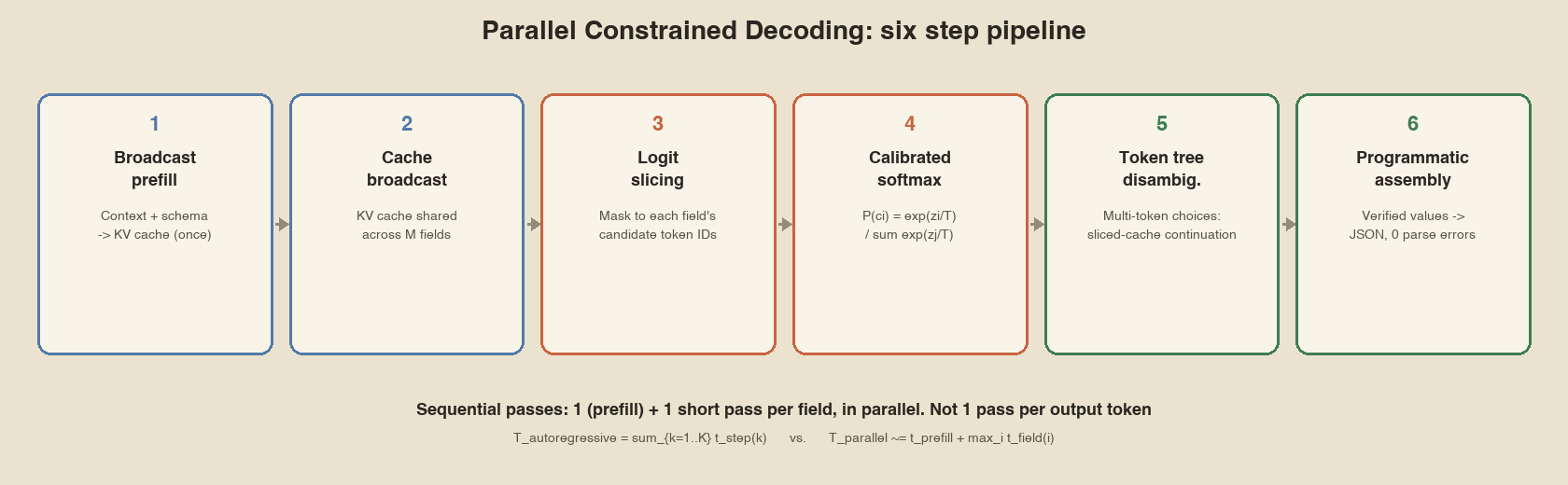
Fig. 1: The six stage pipeline. Stages 1 and 2 run once per request. Stages 3 to 5 run once per field, independently.
4. The algorithm
- Broadcast prefill. Put the context and the schema field descriptions through the model once. Store the KV cache.
- Cache broadcast. Share that one KV cache with all \(M\) fields. No field reprocesses the context.
- Logit slicing. For each field, run a short pass over its own suffix tokens. Read only the logits at that field's candidate token IDs. Ignore the rest of the vocabulary.
- Calibrated softmax. Turn the sliced logits into probabilities: \[ P(c_i) = \frac{\exp(z_i / T)}{\sum_{j=1}^{C} \exp(z_j / T)} \] \(z_i\) is the logit of candidate \(i\), \(C\) is the number of candidates, \(T\) is temperature.
- Token tree disambiguation. If candidates span several tokens and share a prefix, run extra steps on sliced cache states to tell them apart. No cache reallocation.
- Programmatic assembly. Build the output JSON in code from the chosen values. No parsing of generated text.
Why each stage exists
| Stage | What breaks without it |
|---|---|
| 1. Broadcast prefill | Every field would reprocess the full context. Cost grows with field count. |
| 2. Cache broadcast | Attention would be recomputed for the context on every field. |
| 3. Logit slicing | The top token could be outside the schema. Nothing enforces valid answers. |
| 4. Calibrated softmax | Raw logits are not probabilities. Code cannot threshold them. |
| 5. Token tree step | Candidates with the same first token could not be told apart. |
| 6. Programmatic assembly | Generated JSON text can be malformed. Validity is lost. |
Reference pseudocode
def parallel_constrained_decode(context, schema, model, T=1.0):
    # Stages 1-2: one prefill, one shared KV cache
    kv_cache = model.prefill(context + schema.render_descriptions())

    results = {}
    for field in schema.fields:              # independent, parallelizable
        # Stage 3: short pass reusing the cache, then slice logits
        logits = model.forward(field.suffix_tokens, cache=kv_cache)
        sliced = logits[field.candidate_token_ids()]

        # Stage 4: softmax over the slice only
        probs = softmax(sliced / T)

        # Stage 5: multi token candidates
        if field.has_multi_token_candidates():
            probs = resolve_token_tree(field, kv_cache, probs)

        results[field.name] = {
            "value": field.candidates[argmax(probs)],
            "prob": max(probs),
        }

    # Stage 6: build JSON in code
    return assemble_json(results)
Notes on the softmax
- Normalized over the slice only. Probabilities sum to 1 across the field's candidates, not the full vocabulary. Do not compare them with full vocabulary probabilities.
- Temperature changes confidence, not the answer. Softmax keeps the ranking, so the argmax is the same for any \(T > 0\). Only the reported probability changes.
- Masking detail. Implementations often set non candidate logits to \(-\infty\) instead of gathering. The result is identical because \(\exp(-\infty) = 0\).
- Ties are not covered by the public spec. Add your own tie break rule.
A worked example with two candidates. A boolean field has logits 4.1 for true and 1.8 for false. At \(T = 1\):
At \(T = 2\), the same logits give a flatter result, around 0.76 and 0.24. The chosen answer, true, does not change at either temperature. Only how confident the returned number says the model is changes.
How candidate token IDs are found
Before any scoring happens, each field's allowed answers must be mapped to token IDs once, when the schema is built, not on every request:
- Tokenize each candidate string with the model's own tokenizer.
- If a candidate tokenizes to exactly one token, record that ID. This is the fast path logit slicing uses directly.
- If a candidate tokenizes to more than one token, it needs the token tree step (stage 5) at scoring time, since a single logit lookup cannot resolve it.
- Candidates sharing a first token, such as
BILLINGandBILLING_DISPUTE, are exactly the case stage 5 exists for.
5. Complexity
| Property | Autoregressive | PCD |
|---|---|---|
| Sequential passes | \(K\) (150 to 500 typical) | 1 (the prefill) |
| Latency | \(\sum_{k=1}^{K} t_{\text{step}}(k)\) | \(t_{\text{prefill}} + \max_i t_{\text{field}}(i)\) with full parallelism |
| Growth with field count | Roughly linear | Sub linear. Each field adds one small pass |
| Generated tokens | Length of the JSON | 0 |
| Syntax validity | Not guaranteed | Guaranteed by construction |
In the reference benchmark, going from 4 fields to 28 fields raised the autoregressive output from about 148 tokens to about 312. The PCD speedup improved from 5.6x to 7.0x, because the fixed prefill is a smaller share of the alternative.
The "with full parallelism" condition in the table matters. If the hardware or runtime evaluates fields one after another instead of concurrently, total latency becomes \(t_{\text{prefill}} + \sum_i t_{\text{field}}(i)\), the sum over all fields rather than the slowest one. The published M4 Max numbers reflect whatever concurrency the MLX reference implementation actually achieves on that hardware, not a theoretical best case. Either way, the key property holds: field cost does not compound with generated token length the way autoregressive cost does.
Worked example
Published numbers for the 28 field triage scenario:
- Autoregressive: 1,894.2 ms for 312 tokens, about 6.07 ms per token.
- PCD: 268.4 ms total, one sequential pass.
A separate 3 field example response reports elapsed_ms: 74.5, prefill_ms: 52.1, suffix_eval_ms: 18.2. That is about 70% prefill and 24% field evaluation.
Applying that ratio to the 28 field run is an estimate, not a measurement: roughly 188 ms prefill and 65 ms for all fields, so about 2 to 3 ms per field. The published data has no per field timing for that scenario.
6. Schema specification
from core.schema import StructuredSchema, FieldDefinition

schema = StructuredSchema({
    "priority": {
        "type": "enum",
        "choices": ["P0_CRITICAL", "P1_HIGH", "P2_NORMAL", "P3_LOW"],
        "description": "Urgency tier based on customer business impact"
    },
    "requires_escalation": {
        "type": "boolean",
        "description": "Whether an on-call engineer must be notified"
    },
    "department": {
        "type": "enum",
        "choices": ["BILLING", "INFRASTRUCTURE", "SECURITY", "PRODUCT_SUPPORT"],
        "description": "Target handling department"
    }
})
Fields can also be built explicitly through FieldDefinition, which is the form to use when choices are generated at runtime rather than hand written, such as a tariff code list pulled from a database:
from core.schema import FieldDefinition

tariff = FieldDefinition(
    name="tariff_classification",
    field_type="enum",
    description="Harmonized System 6-digit tariff category code",
    choices=["0101.21", "0101.29", "8471.30", "8517.12", "8542.31"]  # up to 255
)| Constraint | Value |
|---|---|
| Field types | boolean, enum |
| Max choices per enum | 255 |
| Nesting | Not supported. Flat schemas only |
| Cross field dependency | Not supported. Fields are scored independently |
| Free text fields | Not supported |
7. Running it and reading the output
from core.engine import run_parallel_generation

result = run_parallel_generation(context, schema)
print(result["elapsed_ms"], result["sequential_forward_passes"])
print(result["parsed_json"])
Response shape:
{
  "mode": "parallel_constrained_calibrated",
  "elapsed_ms": 74.5,
  "prefill_ms": 52.1,
  "suffix_eval_ms": 18.2,
  "sequential_forward_passes": 1,
  "is_valid_json": true,
  "schema_match": true,
  "parsed_json": {
    "priority": { "value": "P0_CRITICAL", "prob": 0.9924 },
    "requires_escalation": { "value": "true", "prob": 0.9981 },
    "department": { "value": "INFRASTRUCTURE", "prob": 0.9815 }
  },
  "field_telemetry": {
    "priority": {
      "confidence": 0.9924,
      "cardinality": 4,
      "top_choices": [
        { "choice": "P0_CRITICAL", "probability": 0.9924 },
        { "choice": "P1_HIGH",     "probability": 0.0068 }
      ]
    }
  }
}
sequential_forward_passes: 1means the whole request had one sequential dependency.field_telemetryexposes the full distribution, so your code can apply its own confidence threshold.
A typical use of field_telemetry is routing low confidence answers to a human or to a larger model instead of trusting every automated decision equally:
result = run_parallel_generation(context, schema)
for name, field in result["parsed_json"].items():
    if field["prob"] < 0.75:
        send_for_human_review(name, field["value"], field["prob"])
    else:
        apply_automatically(name, field["value"])
This pattern, a confidence threshold deciding between automatic action and escalation, is the same cascade idea used by cheap LLM judges: accept confident answers, send the rest somewhere more expensive or more careful.
8. Benchmark data
Apple Silicon M4 Max, mlx-community/Qwen2.5-1.5B-Instruct-4bit, macOS Sequoia.
| Scenario | Fields | Autoregressive | PCD | Speedup |
|---|---|---|---|---|
| Fintech fraud routing | 4 | 420 ms | 75 ms | 5.6x |
| Code security audit | 4 | 380 ms | 68 ms | 5.6x |
| Tariff classification | 1 field, 255 choices | 500 ms | 89 ms | 5.6x |
| Enterprise support triage | 28 | 1,900 ms | 270 ms | 7.0x |
Raw CLI output from the same runner:
Fintech Fraud Detection (4 fields)
  Autoregressive :  421.3 ms | 148 tokens | Passes: 148
  Parallel       :   74.8 ms |   0 tokens | Passes: 1
  SPEEDUP: 5.6x (step reduction 148x)

Support Triage Matrix (28 fields)
  Autoregressive : 1894.2 ms | 312 tokens | Passes: 312
  Parallel       :  268.4 ms |   0 tokens | Passes: 1
SPEEDUP: 7.1x (step reduction 312x)What this means for throughput, not just latency
Latency per request is one axis. The other is how many requests a single machine can serve per second, which matters more for a high volume classification endpoint than for a one-off call. Because PCD replaces 148 to 312 sequential forward passes with 1, a server handling many concurrent requests spends far less total compute per request, which directly raises how many requests the same hardware can serve before it needs to scale out. The published benchmarks report single-request latency only; they do not report a throughput or requests-per-second figure, so treat the throughput gain as directionally implied by the step count reduction, not as a measured number.
9. Compared with other structured output methods
| Method | How it decodes | Valid syntax | Sequential passes |
|---|---|---|---|
| Plain JSON prompting | Autoregressive, unconstrained | No | \(K\) |
| Grammar constrained decoding | Autoregressive, each token masked to grammar valid tokens | Yes for syntax | \(K\) |
| PCD | Prefill once, score candidates per field | Yes, by construction | 1, plus \(M\) independent field passes |
Grammar constrained decoding still generates token by token. It limits what each token may be, but it still needs one forward pass per token. PCD removes the generation loop for field values.
The two can be combined in principle: PCD for bounded fields, another method for free text. The public PCD code does not support free text fields.
PCD versus speculative decoding
These solve different problems and are easy to confuse because both claim to cut the number of real forward passes.
| Speculative decoding | PCD | |
|---|---|---|
| Output space | Open ended text, any length | A fixed set of candidates per field |
| How it saves passes | A small draft model guesses several tokens, the big model verifies them in one pass | Candidates are scored directly, nothing is generated |
| Needs a second model | Yes, a draft model | No |
| Guarantees valid output | No more than normal decoding does | Yes, by construction |
10. Building it yourself
None of this needs proprietary infrastructure. The pieces are standard parts of any modern inference stack:
- Pick a model that exposes logits, not just sampled text. Any local Hugging Face model, or an API that returns logprobs, qualifies.
- Tokenize every candidate answer once, at schema build time, and record which are single token and which need the token tree step.
- Prefill the context and keep the KV cache, using whatever cache API your inference library already exposes for normal autoregressive generation.
- For each field, run one short forward pass reusing the cache, slice the logits to the candidate IDs, and softmax.
- Assemble the output in code, never by asking the model to produce the final JSON string.
Harsha Gundala's repository and Bespoke Labs' Nimble are both working reference implementations of exactly this recipe, in Python, and are the fastest way to see it running before writing your own version.
11. When to use it
| Your output | Use PCD? |
|---|---|
| All fields are booleans or fixed enums | Yes. This is the target case. |
| Some fields need free text | Not for those fields. Route them elsewhere. |
| One field's choices depend on another field | Not in one call. Use two calls or filter the distribution in code. |
| Nested objects or arrays | No. Schemas must be flat. |
| More than 255 choices in one field | Not directly. Bucket or split the decision. |
Edge cases worth planning for
| Situation | What to do |
|---|---|
| None of the candidates actually fit the input | Add an explicit "none of the above" or "not stated" choice to the field. Without one, the model is forced to pick the least-wrong option and the probability on it will usually be low, which your confidence threshold should catch. |
| A field's correct answer genuinely requires context from another field | Split into two calls: resolve the first field, then pass its value into the context for a second call that resolves the dependent field. |
| Candidate list changes often, such as a product catalog | Use FieldDefinition with choices generated at request time rather than hard coding a static schema, and re-tokenize whenever the list changes. |
| You need an explanation alongside the decision | PCD cannot produce one. Log the full probability distribution and, if a reason is required, pair the decision with a separate, normal generative call only when needed. |
12. Limits
- No free text and no nesting in the reference implementation. A field that needs a short explanation, a summary, or a verbatim quote from the context cannot be expressed in this schema format at all.
- No cross field conditioning inside one call. If field B's valid choices should depend on what field A returned, that dependency has to be enforced by your own code after the fact, or split into two sequential calls.
- 255 choice ceiling per enum. Multi token choices need the extra token tree step, which costs more than single token choices, so a schema built entirely from long, multi-word candidate strings will not see the full benchmarked speedup.
- Apple Silicon only in the published engine. The idea works on any stack that exposes logits and KV cache reuse, but the benchmark numbers are specific to MLX on an M4 Max and have not been reproduced on CUDA or other hardware in the public material this reference is built from.
- Valid is not correct. PCD guarantees a valid output. It does not guarantee the chosen answer is right. The public benchmarks report latency and validity, not task accuracy, so accuracy on your own data needs its own evaluation.
- No built in explanation. The output is a value and a probability, never a reason. If your workflow needs "why did it pick this," that has to come from a separate system, such as logging the full candidate distribution for later review.
ParallelScorer on Apple Silicon processes the context once and scores all fields. Its CUDA scorer scores each field with the full prompt, so it skips the cache sharing. Nimble also says fields cannot see each other's answers.How this relates to Jev
PCD is the mechanism several independent sources use to explain how TypeSafe's Jev model likely works internally, though TypeSafe itself has never confirmed an architecture. The match is based on matching behavior: Jev's 70 to 500 millisecond latency, its free output tokens, and its guaranteed valid output all follow directly from this kind of scoring based pipeline rather than generation. See How Jev Actually Works for the full reverse engineering writeup, including a side by side accuracy comparison against an open model trained the same way.
13. Debugging and common errors
Most problems people hit with PCD are not model problems. They come from schema definition, tokenization, or a mismatch between the candidate strings and what the model actually emits. The table below lists the failures seen most often and how to narrow each one down.
| Symptom | Likely cause | How to check |
|---|---|---|
| Every field returns the same top candidate | Candidate strings are tokenized to identical IDs, or the descriptions are not included in the prefill, so the model has no basis to distinguish fields | Print the candidate token IDs for each field. Confirm the prefill string contains each field's description. |
| Probabilities are nearly uniform across all candidates | Temperature is set high, or the model is too small to separate the candidates for this task | Run the same input at a lower temperature. Compare against a larger model on a handful of examples. |
| A multi word enum always resolves to its first word | The token tree step is being skipped, so only the first token of each candidate is scored | Check has_multi_token_candidates() for that field. Confirm the disambiguation branch runs. |
| Schema validation fails on a boolean field | The boolean is returned as the string "true" or "false" rather than a native boolean, which is the case shown in the response example | Convert the string to a boolean in your own parsing layer, since the engine returns string values inside the JSON. |
| Latency is higher than the published benchmark | The schema has many long multi token candidates, or the context is much longer than the benchmark prompts | Measure prefill and suffix time separately using prefill_ms and suffix_eval_ms from the response. |
| A candidate outside the list appears in output | Output was assembled from raw generated text instead of from the sliced candidates | Verify the assembly step. A correct PCD implementation cannot emit a value outside the declared candidates. |
13.1 A short pre-deployment checklist
- Every enum has at least two candidates and no more than 255.
- Every candidate string tokenizes to the number of tokens you expect. Print the list once and review it.
- Every field has a description that states the question plainly, since the description is part of the prefill.
- An explicit "not stated" or "none of the above" candidate exists on any field where the answer may be absent.
- Confidence thresholds are chosen on labeled data from your domain, not copied from a benchmark.
- Latency is measured on your real context lengths, with prefill and per field time logged separately.
- Accuracy is measured on a held out labeled set, since validity alone does not show that the chosen answers are right.
14. A complete request, end to end
This section walks through one realistic request from schema definition to the value an application acts on. It uses the same three field schema as the earlier examples so the numbers are consistent across the article.
Step 1: the context. A support ticket arrives: a payment gateway is failing for a large share of checkout attempts, and the account is a high tier enterprise customer. The text is passed in unchanged. No preprocessing into a special format is needed.
Step 2: the schema. Three fields are defined: a four level priority enum, a boolean for whether an on call engineer must be paged, and a four option department enum. Each has a description written as a plain question. The descriptions are part of the prefill, so their wording is part of the model's input.
Step 3: the prefill. The context and the three descriptions are processed once. The KV cache now holds everything the three field passes need. This is the only pass over the full context.
Step 4: the field passes. Each field gets a short forward pass over its own suffix tokens, reusing the cache. For the priority field, the four candidate logits are read and softmaxed. The same happens for the other two fields, independently.
Step 5: assembly and return. The engine builds the JSON from the chosen values and returns the telemetry shown in section 7. In the response shape, sequential_forward_passes is 1, which records that the request had one sequential dependency, the prefill.
Step 6: the application acts. The application reads the three values and their probabilities. A high confidence paging decision goes straight to the on call system. A low confidence one goes to a human triage queue. The threshold is the only piece of business logic the model call itself does not contain, and it is the piece most worth testing against real tickets.
15. Glossary
| Term | Meaning here |
|---|---|
| Prefill | The forward pass over the input context, before any output is produced. |
| KV cache | The stored key and value tensors from prefill, reused so later passes do not recompute attention over the same context. |
| Logit | A model's raw, unnormalized score for one vocabulary token, before softmax. |
| Logit slicing | Keeping only the logits at a chosen subset of token IDs and discarding the rest. |
| Argmax | The candidate with the highest probability or score. |
| Calibration | Whether a stated confidence, such as 90%, actually matches how often that answer is correct. |
FAQ
Is this speculative decoding?
No. Speculative decoding speeds up open ended generation with a draft model. PCD does not generate field values. It scores a fixed set of candidates.
Can it return a value outside the schema?
No. Logits are sliced to the field's candidate token IDs, so the argmax can only be one of them. This guarantees schema validity. It says nothing about whether the value is correct.
Does more fields always improve the speedup?
In the four benchmarks, yes: 5.6x at 4 fields, 7.0x at 28. It is not unbounded. Each field still costs a small pass, and the benchmarks stop at 28 fields.
Where can I try it without installing?
The model card links a hosted demo: drinkmoonshine/parallel-constrained-decoding on Hugging Face Spaces.
Does the model need special training to support this?
No. The published technique runs on a stock instruction tuned model with no fine tuning. Training can improve accuracy and calibration on top of it, but the mechanism itself works on an off the shelf model.
What happens if two candidates get the exact same score?
The public specification does not define tie breaking behavior. In practice, floating point ties are rare but not impossible, especially at low temperature on a small model. Pick a deterministic rule, such as the first candidate in declaration order, and apply it consistently in your own code.
Is this the same as adding a classification head to the model?
No. A classification head is a separate trained layer bolted onto the model, specific to one task, usually requiring its own training run. PCD reuses the model's existing, general purpose language modeling head and vocabulary. The same base model can answer any new schema you define without retraining anything.
Takeaways
- PCD swaps generation for scoring on bounded fields.
- \(K\) sequential passes become 1 prefill plus \(M\) small independent passes.
- Valid syntax is guaranteed. Correctness is not, so accuracy still needs its own evaluation on your data.
- It is not grammar constrained decoding, which still loops per token, and it is not speculative decoding, which needs a second draft model.
- No training is required to get the speedup. Training only improves accuracy and calibration on top of it.
field_telemetry's full probability distribution is what makes a confidence-threshold cascade to human review or a bigger model possible.- Limits: flat schema, no free text, no cross field dependency in one call, 255 choices per field, no built in explanation, and published benchmarks specific to Apple Silicon.
References
Primary sources for every claim, formula and number in this reference document:
- harshatheg/Qwen-2.5-1B-RLCD on Hugging Face Primary source for the algorithm, formulas, API and benchmarks.
- Live side by side demo Runs in the browser.
- Harsha Gundala, release announcement Original context.
- bespokelabsai/nimble Independent implementation of the same pattern.
- How Jev Actually Works Applied context and the MiniCheck lineage.
- System One Models and Jev Original technical read on the Jev launch.